
Vaizdas:Lens and wavefronts.gif
Nėra didesnės raiškos varianto.
Lens_and_wavefronts.gif (183 × 356 taškų, rinkmenos dydis: 35 KiB, MIME tipas: image/gif, ciklinis, 9 kadrai, 0,7 s)
| Ši byla yra iš bendros Wikimedia Commons nemokamų resursų duomenų bazės, palaikomos Wikimedia Foundation organizacijos. Norėdami sužinoti licencijavimo smulkmenas, žiūrėkite paveikslėlio aprašymą |  |
Į paveikslėlio aprašymą |
slnglelens
Aprašymas
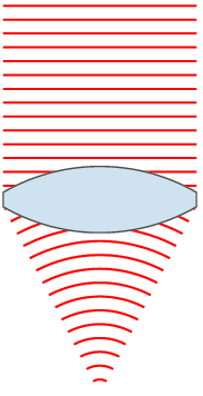
| Aprašymas | Illustration of wavefronts after passing through a lens. Interestingly, to produce a point source reverse the direction of the waves, with the focus point acting as a point source. |
| Data | (UTC) |
| Šaltinis | self-made with MATLAB |
| Autorius | Oleg Alexandrov |
| Kitos versijos |
 |
Šis GIF paveikslėlis sukurtas su MATLAB.
Licencija
| Aš, šio darbo autorinių teisių savininkas, šį darbą skelbiu viešo naudojimo. Tai galioja visame pasaulyje. Kai kuriose šalyse tai negali būti legaliai leidžiama; jei taip: Suteikiu teisę naudoti šį darbą bet kokiai paskirčiai, be jokių sąlygų, nebent jos reikalaujamos įstatymų. |
siingleline
% Illustration of planar wavefronts going through a lens and getting focused
% into a converging spherical wave

function main ()

  % lens index
   n=1.5;

  % number of points, used for plotting
   N = 100;

  % radii of lens surfaces
   R1 = 0.5;
   R2 = 1.5;

  % centers of circles (y coord is 0)
   O1 = -2.9;
   O2 = -O1;

  % focal length
   f = (n-1)*(1/R1+1/R2); f = 1/f;

   % theta0 determines the width of the lens
   theta0=pi/6;
   Theta = linspace(-theta0, theta0, N);

  % right face of the lens
   L1x = R1*cos(Theta)+O1;
   L1y =R1*sin(Theta);

   % left size of the lens
   L2x=-R2*cos(Theta)+O2;
   L2y = R2*sin(Theta);

   % flat top part
   Topx = [L1x(N), L2x(N)];
   Topy = [L1y(N), L2y(N)];

   % flat bottom part
   Botx = [L1x(1) L2x(1)];
   Boty = [L1y(1), L2y(1)];

   % the lens
   Lensx = [L1x rv_vec(Topx), rv_vec(L2x), Botx];
   Lensy = [L1y rv_vec(Topy), rv_vec(L2y), Boty];

   % Parameters for graphing
   Lens_color  = [204, 226, 239]/256;
   Lens_border = 0.3*[1, 1, 1];
   lbw = 1.3; % lens border width
   wavefr_color = [1, 0, 0];
   wavefr_bdw   = 2;

   % spacing between wavefronts (both plane and spherical ones)
   spacing = 0.25;

   % 2*H is the height of the plane wavefronts
   H = L1y(N);

   % theta2 = slope of the line going from the upper-right
   % end of the lens to the focus point
   theta2 = atan(L1y(N)/(f-L1x(N)));

   % Shape of the spherical wavefronts.
   Theta = linspace(-theta2, theta2, N);
   X = -cos(Theta);
   Y =  sin(Theta);

   S = -f; % start ploting waves from here to the right

   % number of frames in the movie
   num_frames = 10;
   Shifts = linspace(0, spacing, num_frames+1);

   % start at S+shift, plot the wavefronts
   for frame_no = 1:num_frames

      shift = Shifts(frame_no);

      s = S+shift;

      % plotting window
      figure(1); clf; hold on; axis equal; axis off;

      % plot the plane wavefronts
      while s < 0
         plot([s, s], [-H, H], 'color', wavefr_color, 'linewidth', wavefr_bdw);
         s = s + spacing;
      end


      % plot the spherical wavefronts
      s = s - 10*spacing; % backtrack a bit
      while s < f

         rho = f-s;

         if rho*Y(N) <= L1y(N)
            plot(rho*X+f, rho*Y, 'color', wavefr_color, 'linewidth', wavefr_bdw);
         end

         s = s + spacing;

      end

      % plot the lens
      fill(Lensx, Lensy, Lens_color, 'EdgeColor', Lens_border, 'LineWidth', lbw);
%      get(H)
%      return

      % Invisible points to force MATLAB to keep the
      % plotting window fixed.
      tiny = 0.15*spacing;
      white = 0.999*[1, 1, 1];
      plot(S-tiny,   H+tiny, 'color', white);
      plot(S-tiny,  -H-tiny, 'color', white);
      plot(f+tiny,   H+tiny, 'color', white);
      plot(f+tiny,  -H-tiny, 'color', white);

      % Rotate by 90 degrees
      set(gca, 'View', [90, 90])

      % save current file
      frame_file = sprintf('Frame%d.eps', 1000+frame_no);
      disp(frame_file);
      saveas(gcf, frame_file, 'psc2');
      pause(0.07)
   end

% The frames were converted to a movie with the command
% convert -antialias -loop 10000  -delay 8 -compress LZW Frame100* Lens_and_wavefronts.gif

function W = rv_vec(V)

   K = length(V);

   W = V;
   for i=1:K
      W(i) = V(K-i+1);
   end
Rinkmenos istorija
Paspauskite ant datos/laiko, kad pamatytumėte rinkmeną tokią, kokia ji buvo tuo metu.
| Data/Laikas | Miniatiūra | Matmenys | Naudotojas | Paaiškinimas | |
|---|---|---|---|---|---|
| dabartinis | 09:35, 25 lapkričio 2007 | | 183 × 356 (35 KiB) | Oleg Alexandrov | tweak |
| 07:10, 24 lapkričio 2007 |  | 171 × 356 (33 KiB) | Oleg Alexandrov | tweak | |
| 07:09, 24 lapkričio 2007 |  | 171 × 356 (33 KiB) | Oleg Alexandrov | tweak | |
| 03:56, 24 lapkričio 2007 |  | 171 × 359 (33 KiB) | Oleg Alexandrov | tweak, same license | |
| 03:53, 24 lapkričio 2007 |  | 171 × 359 (32 KiB) | Oleg Alexandrov | tweak | |
| 03:49, 24 lapkričio 2007 |  | 151 × 359 (31 KiB) | Oleg Alexandrov | {{Information |Description=Illustration of wavefronts after passing through a [:en:lens (optics)|lens]] |Source=self-made with MATLAB |Date=~~~~~ |Author= Oleg Alexandrov |Permission=see below |other_versions= }} |
Paveikslėlio naudojimas
Paveikslėlis yra naudojamas šiuose puslapiuose:
Visuotinis rinkmenos naudojimas
Ši rinkmena naudojama šiose viki svetainėse:
- Naudojama ar.wikipedia.org
- Naudojama ast.wikipedia.org
- Naudojama be.wikipedia.org
- Naudojama bn.wikipedia.org
- Naudojama bs.wikipedia.org
- Naudojama ckb.wikipedia.org
- Naudojama cs.wikiversity.org
- Naudojama cv.wikipedia.org
- Naudojama en.wikipedia.org
- Naudojama en.wikiversity.org
- Naudojama es.wikipedia.org
- Naudojama es.wikiversity.org
- Naudojama eu.wikipedia.org
- Naudojama fa.wikipedia.org
- Naudojama fi.wikipedia.org
- Naudojama fr.wikipedia.org
- Naudojama fr.wikibooks.org
- Naudojama fy.wikipedia.org
- Naudojama ga.wikipedia.org
- Naudojama he.wikipedia.org
- Naudojama hi.wikipedia.org
- Naudojama hr.wikipedia.org
- Naudojama hy.wikipedia.org
- Naudojama id.wikipedia.org
- Naudojama lv.wikipedia.org
- Naudojama ml.wikipedia.org
- Naudojama mn.wikipedia.org
- Naudojama nl.wikipedia.org
- Naudojama pa.wikipedia.org
- Naudojama ru.wikipedia.org
- Naudojama sh.wikipedia.org
- Naudojama si.wikipedia.org
- Naudojama sl.wikipedia.org
- Naudojama sr.wikipedia.org
- Naudojama sv.wikipedia.org
- Naudojama ta.wikipedia.org
- Naudojama te.wikipedia.org
Žiūrėti visuotinį šios rinkmenos naudojimą.